Plotting: multiple backend support#
PlotCollection already uses elements from xrtist.backend, so it’s existing limited features are completely interchangeable between both backends!
Here are some examples:
import arviz as az
import numpy as np
import xarray as xr

from xrtist import PlotCollection, visuals
idata = az.load_arviz_data("rugby")
post = idata.posterior
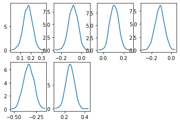
Basic example#
pc = PlotCollection.wrap(
    post["atts"],
    cols=["team"],
)
pc.map(visuals.kde, "kde")
pc = PlotCollection.wrap(
    post["atts"],
    cols=["team"],
    backend="bokeh",
    plot_grid_kws=dict(width=100, height=100)
)
pc.map(visuals.kde, "kde")
show(pc.viz["chart"].item())
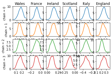
More extense example#
color_cycle = ['#1f77b4', '#ff7f0e', '#2ca02c', '#d62728']
pc = PlotCollection.grid(
    post["atts"],
    cols=["team"],
    rows=["chain"],
    aes={"color": ["chain"]},
    color=color_cycle,
    subplot_kws={"figsize": (12, 8)}
)
pc.map(visuals.kde, "kde")

# once we manually interact with the backend object, we need to adapt
for ax in pc.viz["plot"].sel(chain=0):
    ax.item().set_title(ax["team"].item())


for ax in pc.viz["plot"].isel(team=0):
    ax.item().set_ylabel(f"""chain = {ax["chain"].item()}""")
pc = PlotCollection.grid(
    post["atts"],
    cols=["team"],
    rows=["chain"],
    aes={"color": ["chain"]},
    color=color_cycle,
    backend="bokeh",
    plot_grid_kws=dict(width=100, height=100)
)
pc.map(visuals.kde, "kde")

# once we manually interact with the backend object, we need to adapt
for ax in pc.viz["plot"].sel(chain=0):
    ax.item().title = ax["team"].item()


for ax in pc.viz["plot"].isel(team=0):
    ax.item().yaxis.axis_label = f"""chain = {ax["chain"].item()}"""

show(pc.viz["chart"].item())
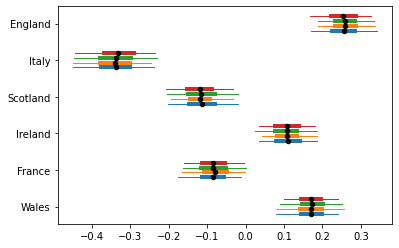
plot_forest mimic#
y = np.arange(6)[:, None] + np.linspace(-.2, .2, 4)[None, :]

pc = PlotCollection.wrap(
    post["atts"],
    aes={"color": ["chain"], "y": ["team", "chain"]},
    y=y.flatten(),
    color=color_cycle,
    subplot_kws={"figsize": (12, 8)}
)
pc.map(visuals.interval, "hdi", linewidth=1)
pc.map(
    visuals.interval,
    "quartile_range",
    linewidth=4,
    interval_func=lambda values: np.quantile(values, (.25, .75))
)
pc.map(visuals.point, "mean", color="black", size=20, zorder=2)

# and here we adapt
pc.viz["plot"].item().set_yticks(np.arange(6), post["team"].values);
y = np.arange(6)[:, None] + np.linspace(-.2, .2, 4)[None, :]

pc = PlotCollection.wrap(
    post["atts"],
    aes={"color": ["chain"], "y": ["team", "chain"]},
    y=y.flatten(),
    color=color_cycle,
    backend="bokeh",
    plot_grid_kws={"subplot_kws": dict(width=600, height=400)}
)
pc.map(visuals.interval, "hdi", linewidth=1)
pc.map(
    visuals.interval,
    "quartile_range",
    linewidth=4,
    interval_func=lambda values: np.quantile(values, (.25, .75))
)
pc.map(visuals.point, "mean", color="black", size=5)

##
yaxis = pc.viz["plot"].item().yaxis.major_label_overrides = {
    k: v for k, v in enumerate(post["team"].values)
}

show(pc.viz["plot"].item())