PlotMuseum overview#
This notebook builds on top of Data organizers: proof of concept to show usage of PlotMuseum class.
import arviz as az
import numpy as np
import xarray as xr
import matplotlib.pyplot as plt
xr.set_options(display_expand_data=False);
az.style.use("arviz-white")
idata = az.load_arviz_data("rugby")
post = idata.posterior
from xrtist import PlotMuseum
PlotMuseum is an attempt to generalize the existing features of PlotCollection to take Dataset inputs.
Thus, the .viz and .dt (previously .ds) are now DataTree objects.
Again, we define our kde_artist to get started:
def kde_artist(values, target, **kwargs):
    kwargs.pop("backend")
    grid, pdf = az.kde(np.array(values).flatten())
    return target.plot(grid, pdf, **kwargs)[0]
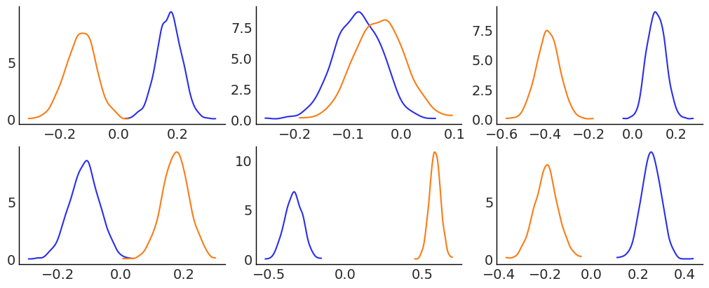
Base example: plot kdes for each of the 6 teams#
We start with a basic example, plotting a kde for each of the teams. In this case, we only want to generate a subplot for each team, no aesthetics or anything else. We indicate this with col=["team"].
Note however that we now have two variables because the input is a Dataset, therefore, even though we provide no aesthetics, as we plot multiple lines in the same plot, matplotlib uses the default prop_cycle to distinguish the lines
pc = PlotMuseum.wrap(
    post[["atts", "defs"]],
    cols=["team"],
    col_wrap=3,
    plot_grid_kws={"figsize": (10, 4)}
)
pc.map(kde_artist, "kde")
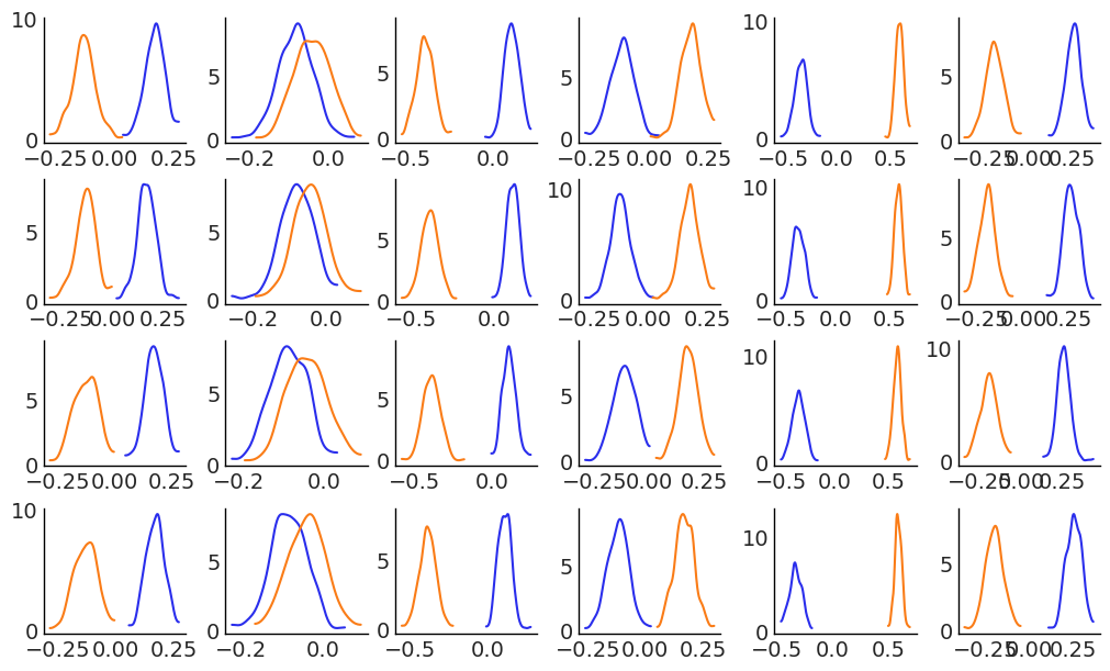
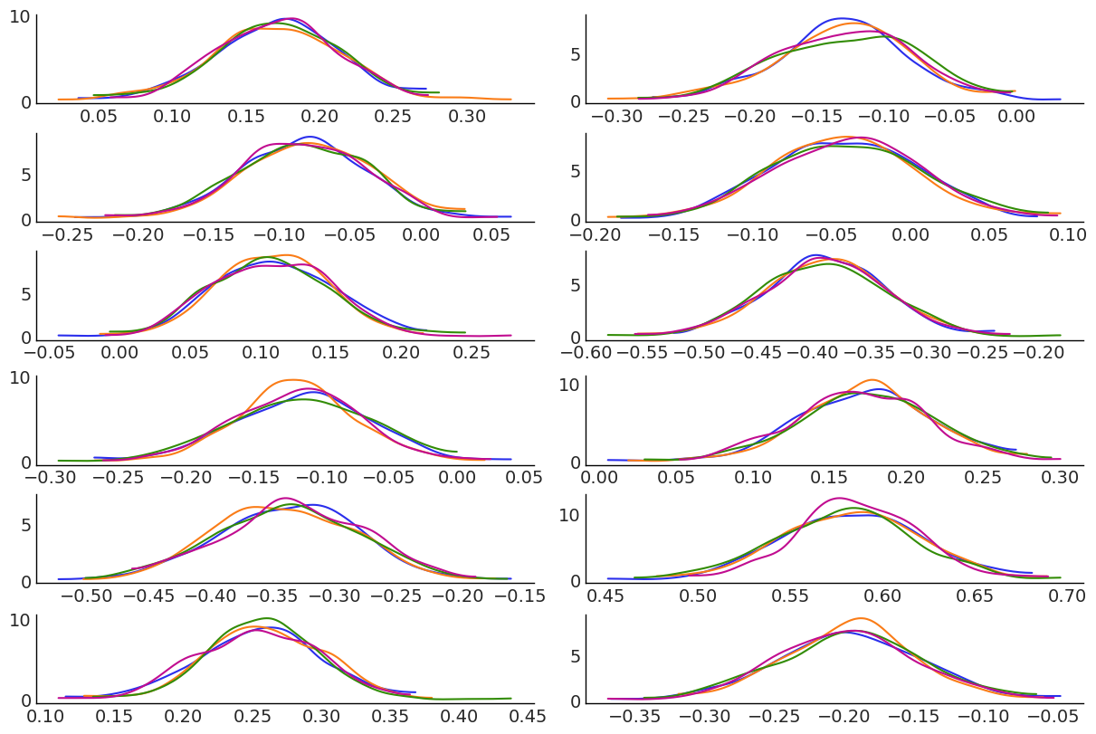
2d grid example#
pc = PlotMuseum.grid(
    post[["atts", "defs"]],
    cols=["team"],
    rows=["chain"],
    plot_grid_kws={"figsize": (10, 6)}
)
pc.map(kde_artist, "kde")
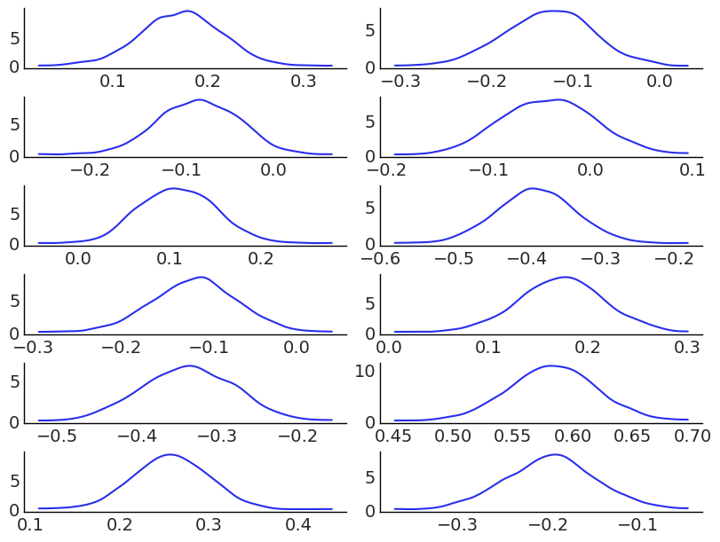
Introduce “variable”#
We can now use "__variable__" string instead of a dimension name to indicate we don’t want to overlay variables but to facet on them.
pc = PlotMuseum.grid(
    post[["atts", "defs"]],
    cols=["__variable__"],
    rows=["team"],
    plot_grid_kws={"figsize": (8, 6)}
)
pc.map(kde_artist, "kde")
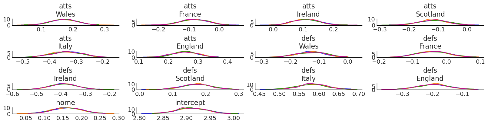
It can be combined with dimensions in order to get the default “concat” style we use in ArviZ, we can also use .wrap:
def title_artist(values, target, var_name, sel, isel, labeller_fun, **kwargs):
    kwargs.pop("backend")
    label = labeller_fun(var_name, sel, isel)
    return target.set_title(label, **kwargs)

pc = PlotMuseum.wrap(
    post[["atts", "defs", "home", "intercept"]],
    cols=["__variable__", "team"],
    col_wrap=4,
    aes={"color": ["chain"]},
    color=[f"C{i}" for i in range(4)],
    plot_grid_kws={"figsize": (16, 4)},
)
pc.map(kde_artist, "kde")
# add title to help visualize what is happening
pc.map(title_artist, "title", subset_info=True, labeller_fun=az.labels.BaseLabeller().make_label_vert, ignore_aes={"color"})
pc.viz
<xarray.DatasetView>
Dimensions:  ()
Data variables:
chart object Figure(1600x400)Or paired with other other facettings and aesthetics:
pc = PlotMuseum.grid(
    post[["atts", "defs"]],
    cols=["__variable__"],
    rows=["team"],
    aes={"color": ["chain"]},
    color=[f"C{i}" for i in range(4)],
    plot_grid_kws={"figsize": (12, 8)}
)
pc.map(kde_artist, "kde")
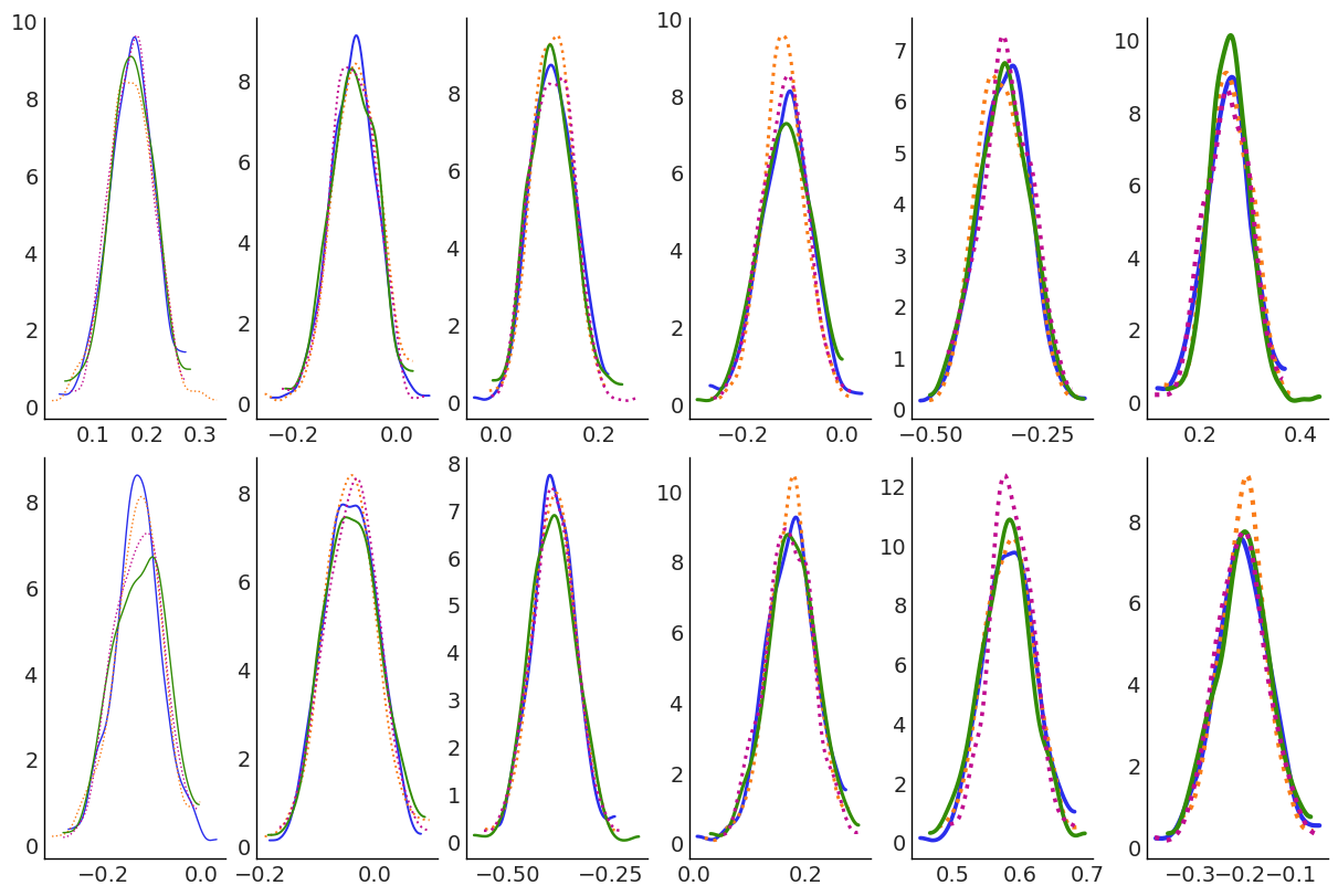
Multiple aesthetics for the same dimension#
We can set multiple asethetics to the same dimension, and both will be updated in sync in all plots:
pc = PlotMuseum.grid(
    post[["atts", "defs"]],
    cols=["team"],
    rows=["__variable__"],
    aes={"color": ["chain"], "ls": ["chain"], "lw": ["team"]},
    color=[f"C{i}" for i in range(4)],
    ls=["-", ":"],
    lw=np.linspace(1, 3, 6),
    plot_grid_kws={"figsize": (12, 8)}
)
pc.map(kde_artist)
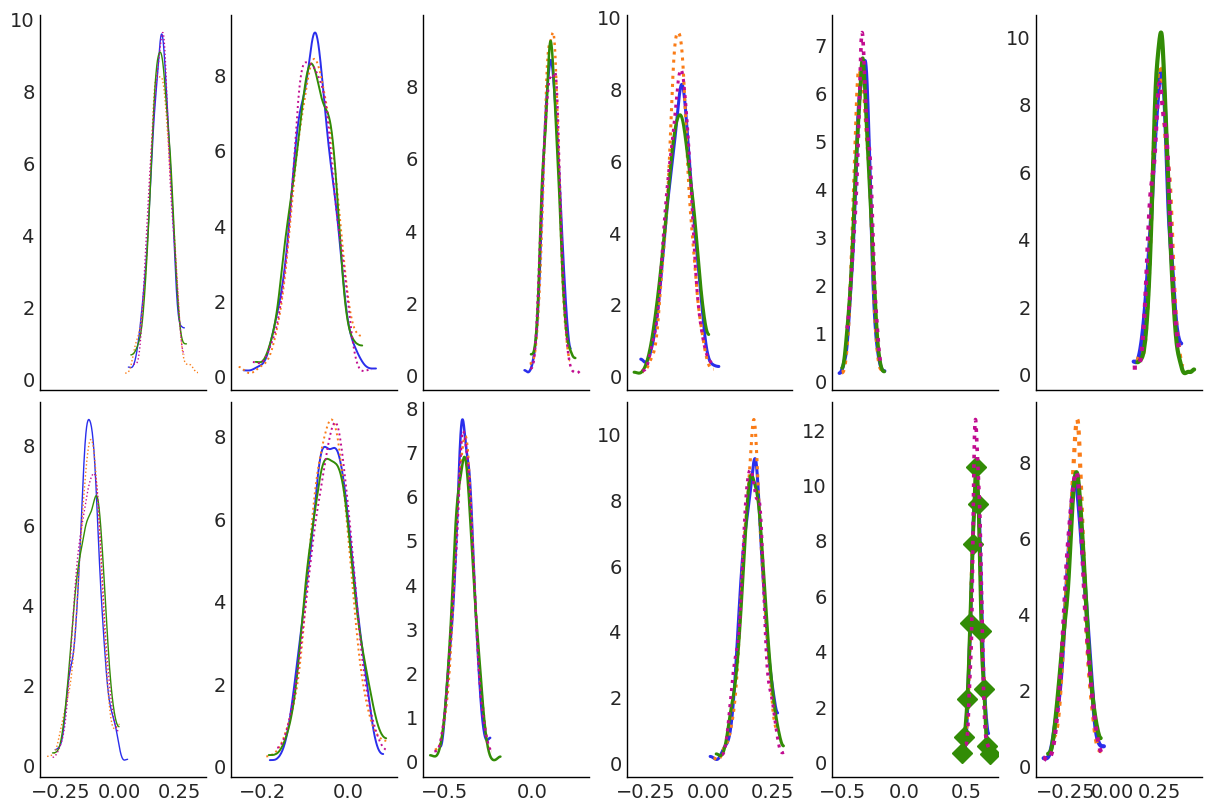
Easy access to all plots elements#
And as we have stored all the plotting related data, including artists in the .viz attribute, we can select artists from the plot and modify them with label based indexing. Here we can make the line for defs of the Italy team and 3rd chain have diamonds as markers after plotting, with size 10 and show markers only once every 50 datapoints.
pc = PlotMuseum.grid(
    post[["atts", "defs"]],
    cols=["team"],
    rows=["__variable__"],
    aes={"color": ["chain"], "ls": ["chain"], "lw": ["team"]},
    color=[f"C{i}" for i in range(4)],
    ls=["-", ":"],
    lw=np.linspace(1, 3, 6),
    plot_grid_kws={"figsize": (12, 8), "sharex": "col"}  # share axis!
)
pc.map(kde_artist, "kde")
pc.viz["defs"]["kde"].sel(team="Italy", chain=2).item().set(marker="D", markersize=10, markevery=50);
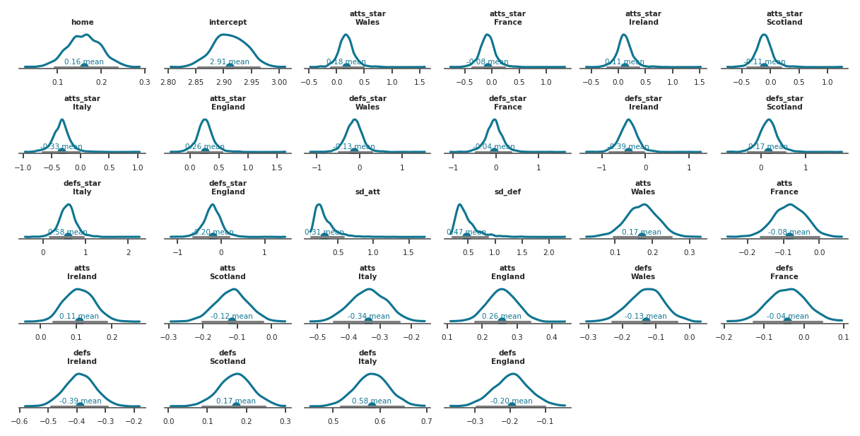
Mimic existing ArviZ functions#
plot_posterior#
We will now mimic plot_posterior. We use functions from the visual module, which generate artists like we did for kde function. We add a couple extras here which are more aesthetic, so they are hidden to not interfere with reading.
Show code cell source
def remove_left_axis(values, target, **kwargs):
    kwargs.pop("backend")
    target.get_yaxis().set_visible(False)
    target.spines['left'].set_visible(False)
We now mimic plot_posterior (dataarray input only). Plot posterior takes an inferencedata and automatically generates the axes and plots everything. With PlotMuseum this now becomes instatiating the class with some defaults (unless one is provided) and then calling .map multiple times to add all the elements to the plot: kde, hdi interval line, point estimate marker, point estimate text…
from xrtist import visuals

def plot_posterior(ds, plot_museum=None, labeller=None):
    if plot_museum is None:
        plot_museum = PlotMuseum.wrap(ds, cols=["__variable__"]+[dim for dim in ds.dims if dim not in {"chain", "draw"}], col_wrap=6, plot_grid_kws={"figsize": (8, 4)})
    if labeller is None:
        labeller = az.labels.BaseLabeller()

    labeller_fun = labeller.make_label_vert

    plot_museum.map(visuals.kde, "kde")
    plot_museum.map(visuals.interval, "interval", color="grey")
    plot_museum.map(visuals.point, "point_estimate", color="C0", size=25, marker="o")
    plot_museum.map(visuals.point_label, "point_label", color="C0", va="bottom", ha="center")
    plot_museum.map(remove_left_axis, store_artist=False)
    plot_museum.map(title_artist, "title", subset_info=True, labeller_fun=labeller_fun)
    return plot_museum
Here it can be seen how the usage is the same basically as our current API, but if we also expose the artist function, it will be much easier for users to create their own variations of plot_posterior or to extend it with their own artist functions.
import matplotlib as mpl
mpl.rcParams.update(mpl.rcParamsDefault)

az.style.use("arviz-doc")
mpl.rcParams["figure.dpi"] = 150
for param in ("figure.titlesize", "axes.titlesize", "axes.labelsize", "xtick.labelsize", "ytick.labelsize", "font.size"):
    mpl.rcParams[param] = 5


pc = plot_posterior(post)
plt.show()
styleFinally, we show how all the elements added to the plot have had their corresponding artists added to the .viz dataset.
pc.viz
<xarray.DatasetView>
Dimensions:  ()
Data variables: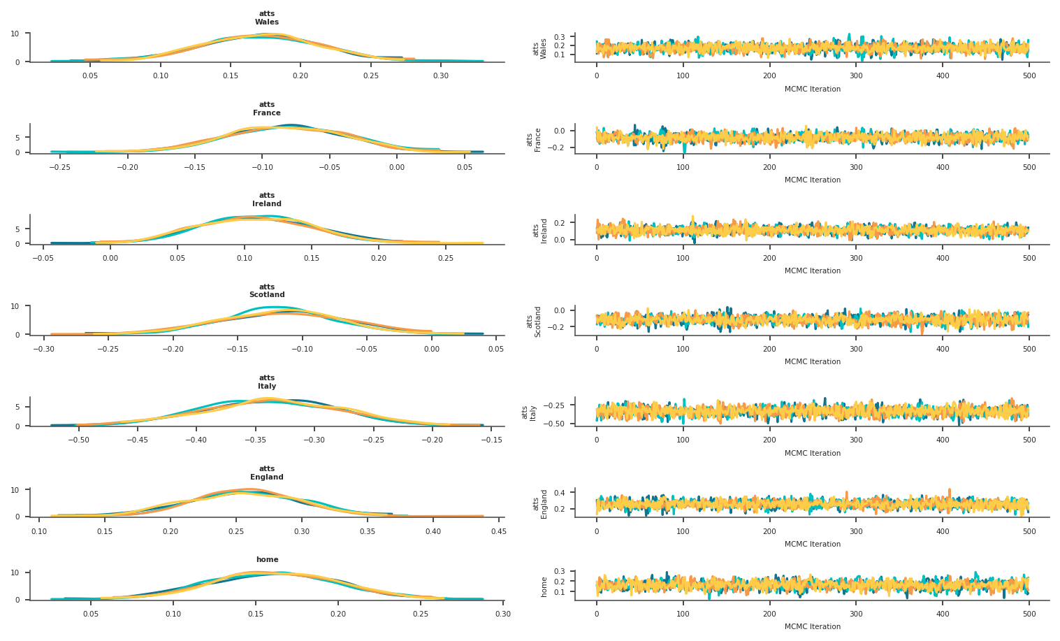
chart object Figure(1200x600)plot_trace#
We will now mimic plot_trace. Here we have an extra keyword compact that defines how we generate the default PlotMuseum,
and we use the coords argument of .map to choose whether to plot on the first or 2nd column. We could as easily use .expand_dims to create
a dim of length 3 and plot kde, trace and rank all side by side…
def line(values, target, backend, **kwargs):
values = np.asarray(values).flatten()
return target.plot(
np.arange(len(values)), values, **kwargs
)[0]
def ylabel_artist(values, target, var_name, sel, isel, labeller_fun, **kwargs):
kwargs.pop("backend")
label = labeller_fun(var_name, sel, isel)
return target.set_ylabel(label, **kwargs)
def xlabel_artist(values, target, text, **kwargs):
kwargs.pop("backend")
return target.set_xlabel(text, **kwargs)
def plot_trace(ds, plot_museum=None, compact=False, labeller=None):
if plot_museum is None:
aux_dim_list = [dim for dim in ds.dims if dim not in {"chain", "draw"}]
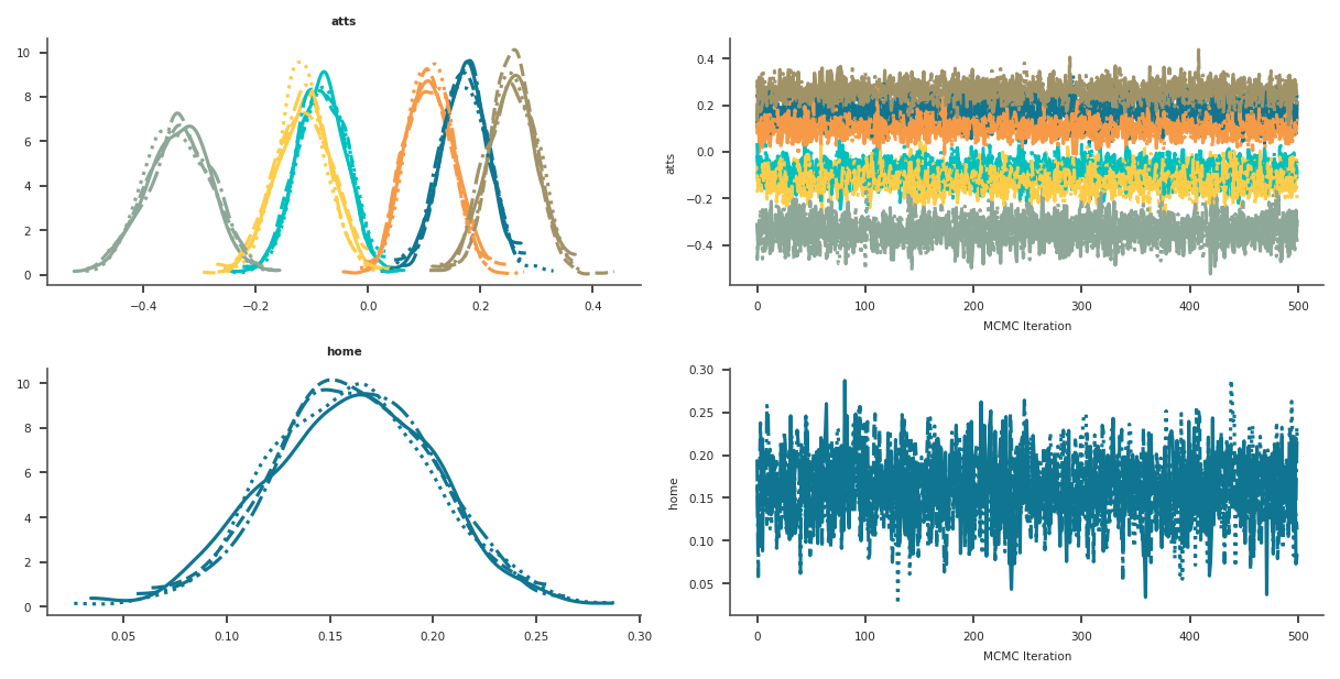
if compact:
# in compact mode, the variable defines the subplot, the coord only defines aesthetics
plot_museum = PlotMuseum.grid(
ds.expand_dims(__column__=2), # add dummy dim for the extra 2 col facetting
cols=["__column__"],
rows=["__variable__"],
aes={"color": aux_dim_list, "ls": ["chain"]},
color=[f"C{i}" for i in range(6)],
ls=["-", ":", "--", "-."],
plot_grid_kws={"figsize": (8, 4)})
else:
# in non-compact mode, the variable+coords define the subplot, only chains are mapped to aesthetics
plot_museum = PlotMuseum.grid(
ds.expand_dims(__column__=2), # add dummy dim for the extra 2 col facetting
cols=["__column__"],
rows=["__variable__"]+aux_dim_list,
aes={"color": ["chain"]},
color=[f"C{i}" for i in range(ds.sizes["chain"])],
plot_grid_kws={"figsize": (10, 6)})
if labeller is None:
labeller = az.labels.BaseLabeller()
labeller_fun = labeller.make_label_vert
plot_museum.map(line, "trace", coords={"__column__": 1})
plot_museum.map(kde_artist, "kde", coords={"__column__": 0})
plot_museum.map(title_artist, "title", subset_info=True, labeller_fun=labeller_fun, coords={"__column__": 0}, ignore_aes={"color", "ls"})
plot_museum.map(ylabel_artist, "xlabel", subset_info=True, labeller_fun=labeller_fun, coords={"__column__": 1}, ignore_aes={"color", "ls"})
plot_museum.map(xlabel_artist, "ylabel", text="MCMC Iteration", coords={"__column__": 1}, ignore_aes={"color", "ls"})
return plot_museum
Note
I generally set ignore_aes to all defined properties for axes labeling artists, as I only want one per subplot,
what about ignore_aes taking either a set or the string "all"?
pc = plot_trace(post[["atts", "home"]])
plt.show()
pc.viz
<xarray.DatasetView>
Dimensions:  ()
Data variables:
chart object Figure(1500x900)pc_compact = plot_trace(post[["atts", "home"]], compact=True)
plt.show()
pc_compact.viz
<xarray.DatasetView>
Dimensions:  ()
Data variables:
chart object Figure(1200x600)Somewhat random plots#
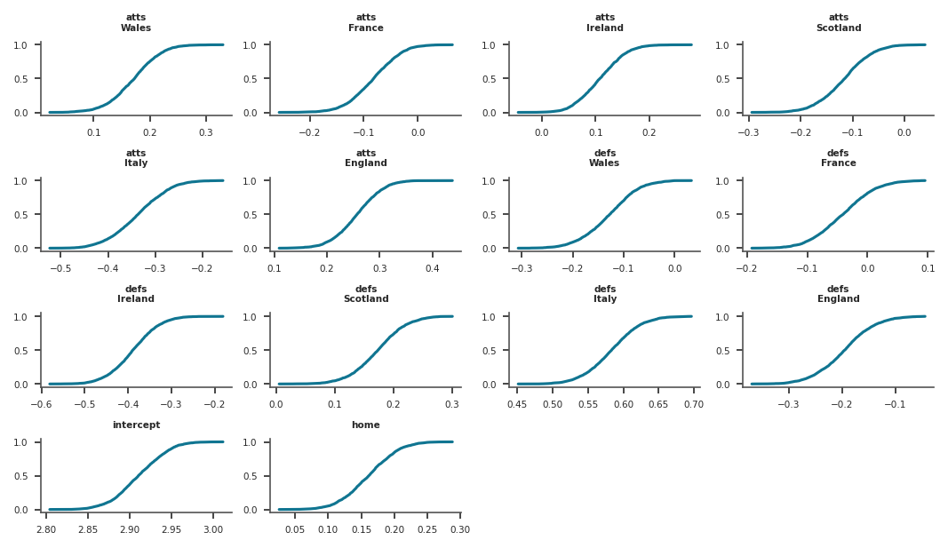
plot_ecdf#
from xarray_einstats.numba import ecdf

def ecdf_line_artist(values, target, backend, **kwargs):
    return target.plot(values.sel(ecdf_axis="x"), values.sel(ecdf_axis="y"), **kwargs)[0]

pc = PlotMuseum.wrap(
    post[["atts", "defs", "intercept", "home"]].map(ecdf, dims=("chain", "draw")),
    cols=["__variable__", "team"],
    plot_grid_kws={"figsize": (7, 4)}
)
pc.map(ecdf_line_artist, "ecdf")
pc.map(title_artist, "title", subset_info=True, labeller_fun=az.labels.BaseLabeller().make_label_vert)
plt.show()
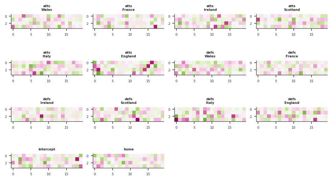
histogram rendered with imshow#
I believe this yet another representation of ranks diagnostic, I think I saw it one day as a potential idea to use when many chains were used.
from xarray_einstats.numba import histogram
from xarray_einstats.stats import rankdata

aux_post = xr.Dataset()
for var_name in ["atts", "defs", "intercept", "home"]:
    aux_post[var_name] = histogram(rankdata(post[var_name], dims=("chain", "draw")), dims="draw", bins=20).rename(
        left_edges=f"{var_name}_left_edges", right_edges=f"{var_name}_right_edges"
    )
aux_post
<xarray.Dataset>
Dimensions:                (team: 6, bin: 20, chain: 4)
Coordinates:
  * team                   (team) object 'Wales' 'France' ... 'Italy' 'England'
    atts_left_edges        (bin) float64 1.0 101.0 200.9 ... 1.8e+03 1.9e+03
    atts_right_edges       (bin) float64 101.0 200.9 300.9 ... 1.9e+03 2e+03
    defs_left_edges        (bin) float64 1.0 101.0 200.9 ... 1.8e+03 1.9e+03
    defs_right_edges       (bin) float64 101.0 200.9 300.9 ... 1.9e+03 2e+03
    intercept_left_edges   (bin) float64 1.0 101.0 200.9 ... 1.8e+03 1.9e+03
    intercept_right_edges  (bin) float64 101.0 200.9 300.9 ... 1.9e+03 2e+03
    home_left_edges        (bin) float64 1.0 101.0 200.9 ... 1.8e+03 1.9e+03
    home_right_edges       (bin) float64 101.0 200.9 300.9 ... 1.9e+03 2e+03
Dimensions without coordinates: bin, chain
Data variables:
    atts                   (team, chain, bin) float64 28.0 23.0 ... 22.0 24.0
    defs                   (team, chain, bin) float64 25.0 24.0 ... 25.0 26.0
    intercept              (chain, bin) float64 29.0 22.0 24.0 ... 32.0 16.0
home (chain, bin) float64 35.0 29.0 28.0 ... 30.0 26.0from matplotlib.colors import LogNorm
def hist_imshow_artist(values, target, backend, **kwargs):
return target.imshow(values, **kwargs)
pc = PlotMuseum.wrap(
aux_post,
cols=["__variable__", "team"],
plot_grid_kws={"figsize": (7, 4)}
)
pc.map(hist_imshow_artist, "hist_imshow", norm=LogNorm(25/2, 25*2), cmap="PiYG")
pc.map(title_artist, "title", subset_info=True, labeller_fun=az.labels.BaseLabeller().make_label_vert)
plt.show()
more to come…